Understand the pipeline

1 - Introduction

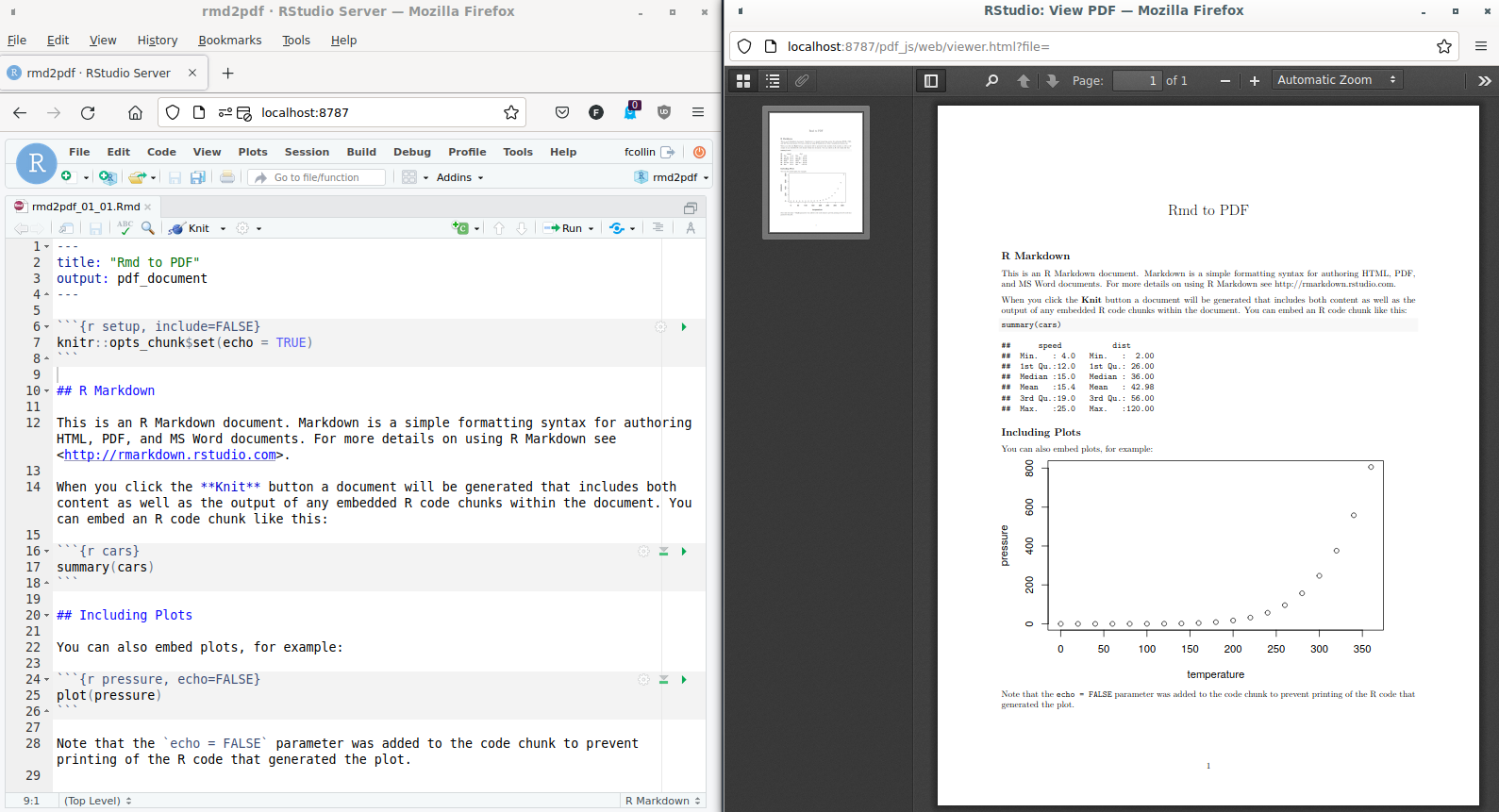
The RStudio environment includes templates of R Markdown documents proposing at selection step to chose PDF output format. It is then easy to render the document, actually simple as a click.

If starting is easy, the click (bait) is hiding complexity as the question of PDF output configuration is more challenging (e.g. add a footnote, change font):

• at least three different nested high-level tools are chained together to handle the R Markdown document (R, Pandoc and a LaTeX engine), fine tuning a PDF document in R consists in passing arguments to the right one using the application interface proposed by R.
• two or three ways exist to convey configuration instructions: either using a R function arguments, or conveying settings via the yaml front matter of the R Markdown document, or eventually through a configuration file.

The aim of the present page is to provide an overview of the tools involved in the pipeline when triggering the rendering of the PDF document, and how to how to pass configuration elements to the right underlying tool.

2. Material and Methods

A series of minimum working examples were generated to support the demonstration. The examples were built at the same time as the results below were reported, they are available as a GitHub repository: Rmd to PDF. Diagrams were employed to describe the sequence of tools involved in the transformation of the R Markdown document to PDF, they were made possible by the Mermaid framework.

The environment for the examples was containerized, a docker image and its definition was used to ensure reproducibility and / or enable the extension of the work (Nüst et al. 2020). The Docker definition was made publicly available at https://github.com/FCACollin/ayup_dock. Note that the image was not originally intended for this specific usage, this explains why it also includes some R packages and LaTeX dependencies not strictly necessary for the examples. However, the image as currently defined was also configured for a research task where pdf reporting was a requirement. Therefore, it was decided to base the example on this image as it shows also how it can be used in production for real-life work.

The image includes:

• A rocker/verse image (4.1.0)
• A series of additional R packages.
• A series of LaTeX dependencies.

In terms of pdf reporting, this image can:

• handles templates.
• use bibliographic references.

3 - Results

3.1 - R Markdown: render()/pdf_document()

Producing a pdf document from a R Markdown (rmd) input is managed by R, but also involves Pandoc: R pre-process all the R Markdown code chunks and in-line code converting there result in markdown and generating an intermediary markdown file (md), Pandoc handles the conversion of the md file into a pdf document. The rmarkdown’s functions render() and pdf_document() are high R level functions which manages most of the features a user might need when generating a report. The options managed by pdf_document() are directly assigned to the right tool to be interpreted simplifying the interaction with the toolchain. For instance, it accepts argument toc resulting in a Table of Content being added to the output, it also accepts keep_md which enables the inspection of the intermediary markdown file.

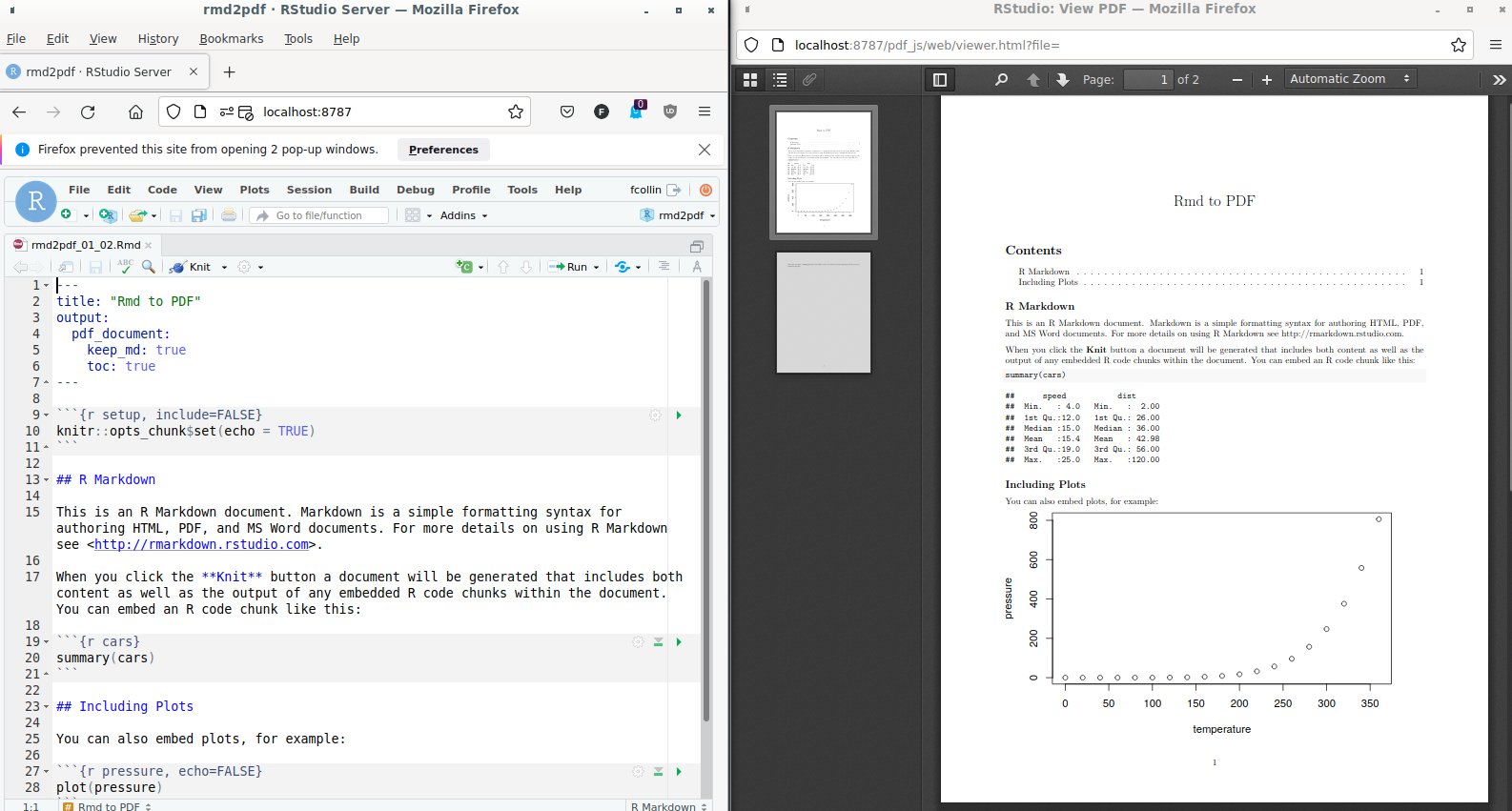
• The options are passed either via the yaml frontmatter (e.g. rmd2pdf_01_03.Rmd) …

  ---
  title: "Rmd to PDF"
  output:
    pdf_document:
      keep_md: true
      toc: true
  ---
  

• … Or via an output function. Comparing both syntaxes, the first line in the yaml front matters below “output” corresponds to the function used by R for configuring the output, (pdf_document) followed by options which find a match in the R function.

  library(rmarkdown)
  render(
    input = "rmd2pdf_01_02.Rmd",
    output_format = pdf_document(toc = TRUE, keep_md = TRUE)
  )
  

3.2 - Pass arguments to Pandoc

R’s function for rendering a pdf document is a high level function. It includes arguments which let the user handle some features of interest for a report, but it is not possible that R’s function accounts for all possibilities offered by the downstream tool Pandoc. This is explained by at list two reasons: Pandoc is highly configurable and proposes a very large number of configuration options, Pandoc is an evolving framework, new features are still to be expected in the future. For Pandoc, configuration of an output is handled by variables for LaTeX . In the example above, the option TOC is conveyed to Pandoc directly. In complement, for the variables which are not directly handled by R’s function (e.g. the font family), the R argument pandoc_args leaves the door opened for more Pandoc variables for LaTeX (e.g. variable fontfamily).

The Pandoc variables for LaTeX can be conveyed via:

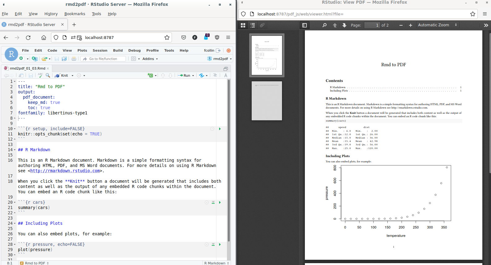
• either the R Markdown document yaml front matter …

  ---
  title: "Rmd to PDF"
  output:
    pdf_document:
      keep_md: true
      toc: true
  fontfamily: libertinus-type1
  ---
  

• … Or the pdf_document() function. Extra lines in the yaml front matter correspond to new pandoc_args list items as built below:

  rmarkdown::render(
    input = "rmd2pdf_01_03.Rmd",
    output_format = rmarkdown::pdf_document(
      toc = TRUE,
      pandoc_args = list(
        "--variable=fontfamily:libertinus-type1"
      )
    )
  )
  

3.3 - Pass arguments to the LaTeX engine

For the same reason which explain why R Markdown can not account for all possibilities offered by Pandoc, Pandoc being a high level function for LaTeX can not account for all possibilities offered by a LaTeX engine. Many expected functionalities are translated via Pandoc, for those which are not, R’s function open the door via the extra dependency argument.

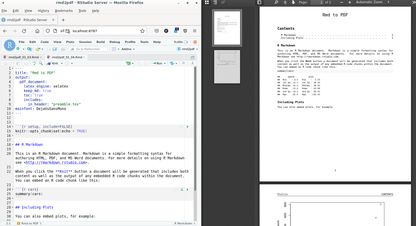
• The yaml front matter is no longer self sufficient, the use of include/in_header points at a supplementary .tex file:
  • yaml:

  ---
  title: "Rmd to PDF"
  output:
    pdf_document:
      latex_engine: xelatex
      keep_md: true
      toc: true
      includes:
        in_header: "preamble.tex"
  mainfont: DejaVuSansMono
  ---
  

  • preambule.tex:

  \usepackage{fancyhdr}
  \pagestyle{fancy}
  \fancyhead[L]{FCollin}
  

• The use of pdf_document() is an interesting alternative, maybe more compact:

  rmarkdown::render(
    input = "rmd2pdf_01_04.Rmd",
    output_format = rmarkdown::pdf_document(
      toc = TRUE,
      latex_engine = "xelatex",
      pandoc_args = list("--variable=mainfont:DejaVuSansMono"),
      extra_dependencies = list(
        rmarkdown::latex_dependency(
          "fancyhdr",
          extra_lines = paste(
            "\\pagestyle{fancy}",
            "\\fancyhead[L]{FCollin}"
          )
        )
      )
    )
  )
  

4. Discussion

It was evidenced that the original raw pdf as generated by a simple click in RStudio, hides complexity. Entering the detail of this complexity and decomposing the pipeline brings a better understanding of the possible levels of configuration which can be addressed either through the R functions, the Pandoc interface or the LaTeX engine. The configuration of the output is also complex and may take advantage of a knowledge of the Pandoc command line interface, a better understanding of the YAML format for configuration, and a basic knowledge of LaTeX may also help in achieving a very well designed report. This complexity allows an incredible flexibility in the configuration of the reporting.

However, the complexity can also be seen as hurdle: the increase number of programming languages decrease the likelihood of finding contributors who can leverage the whole potential of pdf reporting with R Markdown. To alleviate this difficulty it is also possible to use templates: in other word, the configuration of a pdf output is a one-off, it is a deliverable itself which can be injected in many reporting task (think about it as a corporate Microsoft word template).

The pdf reporting as presented above, is an illustration of the mechanisms involved to convert a R Markdown file into a document. The same applies to render docx, html or other: the markdown file being at the cross road and Pandoc involved to the final conversion. As for the pdf documents, all output can take advantage of templates, and markup languages (e.g. LaTeX or html) accepts headers or other additional configuration files.

References

Nüst, Daniel, Vanessa Sochat, Ben Marwick, Stephen J Eglen, Tim Head, Tony Hirst, and Benjamin D Evans. 2020. “Ten Simple Rules for Writing Dockerfiles for Reproducible Data Science.” Public Library of Science San Francisco, CA USA. https://doi.org/10.1371/journal.pcbi.1008316.